

By Lenny Shteyman
If you read my previous article on this subject (“Applying Predictive Analytics for Insurance Assumptions-Setting—When, Why … and Why Not,” May/June 2019), you know that I am a fan of analytics and even a bigger fan of common sense. I do not recommend using predictive models if you can avoid it, which covers most assumptions-setting situations. Since my previous article was published, I have changed roles and learned a few additional lessons from my amazing colleagues that I figured would be worth sharing with the greater actuarial community.
Data-driven underwriting for institutional clients (pensions buyouts, group insurance, reinsurance) is one area where statistical models have been table stakes for a while. This is a great application of predictive analytics, because it meets most of the principles outlined in the previous article: a decent amount of data, multi-dimensionality, major business impact, and need for a repeatable and consistent process. One thing I must make clear: It is still a “small data” exercise, but the lessons learned here are invaluable and can be applied to “big data” as well.
Going forward, I will describe generic situations with examples from the pension risk transfer (PRT) market because I am more familiar with it, but the judgment and philosophy involved are all the same across the spectrum.
Setup
- You are looking to underwrite mortality to price a transaction and you have a few variables for each life that could potentially be predictive. The plan sponsor decided which lives they are sending to you. For example, you might be bidding on everyone in their pension plan who has monthly benefits under $500.
- Underwriting (UW) variables aren’t very sophisticated—they are what’s typically available in the admin system: age, gender, benefit amount, joint and survivor status, mailing ZIP code. There is additional information you might learn through the UW process, such as industry, recent M&A, motivation for the buyout, as well as whether the employees were part time, salaried vs. hourly, or unionized vs. not, etc.
- If you are lucky, you have access to the historical mortality experience of the plan sponsor, which might be exactly applicable or sometimes partially applicable to the group you are underwriting.
- If you are really lucky, you also have access to a much larger “generic” data set of your own historical mortality experience (or purchased from a consulting company) that could significantly enhance your UW decision.
$1 billion question (possible size for a pension transaction): What is the most accurate mortality assumption for pricing this case that you can produce in a reasonable timeline?
Three scenarios will arise:
- Given a lot of plan-specific and relevant mortality data, you might be tempted to ignore the “generic” data set entirely and just build a case-specific mortality model with available variables and use it in pricing.
- With no or a minimal amount of mortality data for the plan, you will need to leverage the larger data set to build a “generic” model for each pricing cell. This is the topic I plan to cover in the majority of this article, but the lessons learned here could also apply to the previous scenario.
- Finally, you might face a scenario where a medium amount of semi-relevant historical experience was provided, and the UW judgment will need to be applied to blend the plan-specific information with the generic model. This scenario is beyond my intended scope.
Key considerations:
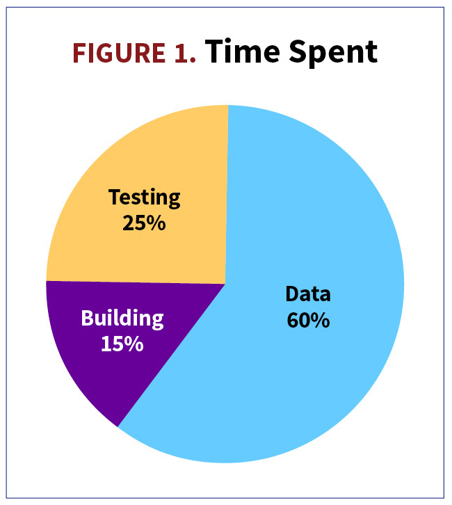
- Data Quality Phase: Sixty percent of your time will be spent on data acquisition, data cleaning, and understanding the data quality and relevance / applicability to the UW process. (See Illustration 1.) It is imperative to recognize data limitations and simple one-dimensional relationships between mortality and drivers before moving forward.
- Model Building Phase: Fifteen percent of your time will be spent on model calibration and experimentation. This is what everyone is commonly excited about when they hear “predictive analytics.” The best advice is to walk before you run and avoid excessive modeling “wizardry” unless the business question absolutely calls for it. As I mentioned before, this is still a “small data” exercise.
- Model Testing Phase: Twenty-five percent of your time will be spent on testing model performance, user acceptance testing with the pricing team, and building stakeholder confidence in your model and documentation. My best advice is to strive for end-user understanding and learn how to explain techniques and observations in plain English.
- Worst-case scenario is spending too much time on model building and too little time on data and testing.
Spoiler alerts:
- Model building for actuarial assumptions is less glamorous than building a model for Google, because you have less data, it is often coming from inconsistent sources, and there is still a lot (!!!) of room for professional actuarial judgment that you cannot delegate to artificial intelligence (AI).
- There is a highly iterative, and often frustrating, nature to the model-building process that cycles between these phases. Something you learn during the model building phase could set you back to the data quality phase; something you learn during model testing could set you back to model building or data quality phases.
- I will give you many interesting questions to ponder, but I am not going to give away all of my answers because the final judgment about your model belongs to you!
5 practical lessons in working with data (Or, it is never as good as you would like):
- Before you begin, you must know what all data fields mean, where they come from, identify most of your data limitations, and be aware of any privacy or regulatory restrictions that would make your data not usable for UW purposes.
- Is your data applicable? Is it consistently collected? Make sure the data is in the same format as will be used in UW. For example, age: exact, nearest birthday, or last birthday. If the UW predictor is not collected at the same time as applied, do you understand a typical drift pattern over time? For example, you might be collecting marital status at the time of retirement or death but applying it at the time of pricing (typically 10 years after retirement and before death)
- How clean is the signal? The signal from PRT variables is typically mixed and, therefore, muted due to offsetting implications for mortality. For example,
a. If someone is single, it could mean never married, married but not electing joint benefit, widowed, or even beneficiary miscoded as retiree.
b. If someone has retired early, it could mean poor health, rich plan provisions, provisions forcing retirement at certain age, or other sources of wealth allowing for early retirement.
c. If someone has a low benefit amount, it could mean they may have low income, had fewer years of service, were a part time worker, or retired a very long time ago when benefits were lower.
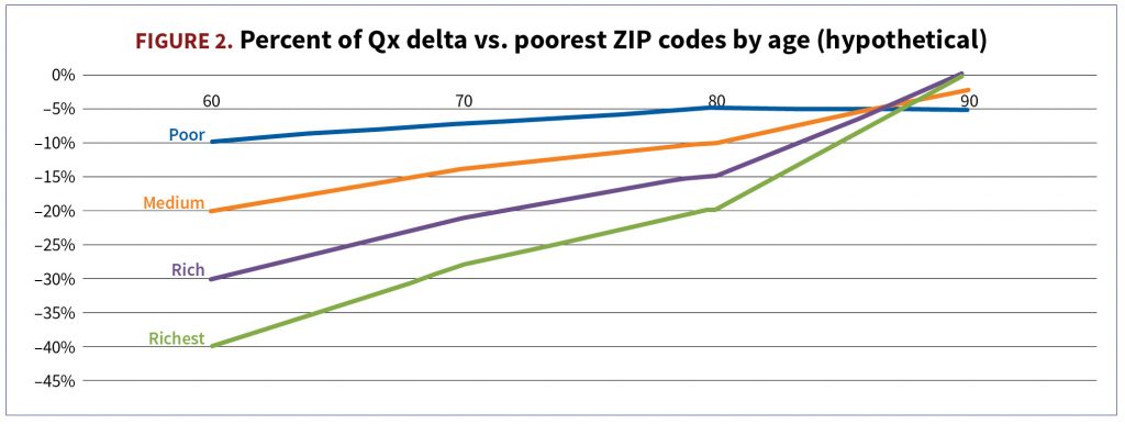
4. Geo variables have gained prominence, but also leave room for judgment. A five-digit ZIP code is less indicative than a nine-digit ZIP code, but the latter might not be available to calibrate a good model. When was the ZIP code information collected—at the time of retirement vs. at the time of pricing? What are you aiming to capture via geo information—economic info (e.g., income), lifestyle info (e.g., smoking probability), historical deaths in a given ZIP code, or all of the above? Does the ZIP code belong to the individual or plan sponsor? Lastly, confirm in your data that effects of socioeconomic factors are not constant. They are typically most pronounced at younger age ranges (ages 60–70) and barely noticeable by more advanced ages (85–90). (See Illustration 2.)
5. What is your plan for 2020 experience? Do you believe COVID-19 excess deaths are predictive of the long-term rates and, if so, to what degree? Do you understand COVID-19 death variability across other predictive dimensions?
5 practical lessons in building a model (wizard vs pragmatic actuary):
- Before you begin, choose your role wisely—avoid playing a statistical wizard (SW) and act as a pragmatic actuary (PA) instead. However, I understand that given the rigorous quantitative training actuaries go through, and emerging popularity of data science as a field, the inner conflict between SW and PA is quite real. Unfortunately, SW can make things complicated very quickly and increase project scope with Day 2 items. For example,
a. If you have salary information, it might be more predictive than benefit amount, because it is less biased. Would you build a model with salary alone or with some combination of salary and pension? What should that combination look like, perhaps Salary + 2 × Benefit? Using both might improve prediction performance metrics but give you less sensible coefficients because salary and pension are correlated, which can lead you on the path of testing and correcting for multi-collinearity. You can easily spend a month analyzing and debating this topic without knowing if it is worth it.
b. If the signal is mixed and could contribute to greater statistical errors, what do you do? For example, you should probably ignore the benefit signal of someone with $25/month pension benefit as nonindicative of mortality, but that is not a good reason to eliminate pension benefit as a variable altogether—or is it?
c. If mean income in a given ZIP code is a relevant variable, is it equally relevant in all scenarios? For example, in some ZIP codes the income variance is low but in others it is high. High variance of income within ZIP code probably implies we should trust the geo information less. Should you find external data that measure income volatility in a given ZIP code? Is that data recent and relevant?
2. Walk before you run. A simpler generalized linear model (GLM)-like model is much more desirable than a very fancy cutting-edge wizardly one, especially because you are aiming to build 30-year mortality predictions, not a real-time automated trading platform. This is easy to convince yourself of by building both models and finding no material improvement in performance due to wizardry.
3. Model segmentation/stratification. The general question is always going to balance the data availability in each segment vs. data relevance across segments. The initial inclination should be vetted with the model users regarding frequency and significance of particular situations to pricing. For example, using gender as a predictor versus building separate models for each gender has a few pros and cons.
a. Arguments for gender as a variable: gender-consistent model will utilize maximum amount of data in calibration and lead to fewer models.
b. Arguments for gender segmentation: genders for the same plan might not be informative of each other and there is also nonconstant gender mix across socioeconomic variables, which will mute the socioeconomic signal if you merge male and female data.
4. What are you going to do for missing or poor-quality predictors? For example, ZIP codes or salary? Will you remove missing ZIP code data from your calibration set (I hope not, because it could create a material bias) or find a way to use all data in the model? Will you attempt wizardry by trying to enrich your missing ZIP code information?
5. How are you capturing mortality improvement? In the predictive model or outside of the model? If in the model, will you use it beyond the historical study period? Should it be based on general population data or target pricing population?
5 practical lessons in model performance and user acceptance testing:
- Before you begin, plan to avoid surprises. Confirm that the pricing team can effortlessly and seamlessly implement your model and use it for future cases. Make sure they believe the model predictions and understand competitive consequences of using your model.
- Does the model make sense? Stay away from excessive wizardry in the model performance department. There are numerous possible performance metrics that will lead to conflicting conclusions. Focus on what makes the most sense to the UW application and pricing exercise. For example,
a. Classical A/E (actual/expected mortality) ratio is your best friend, coming in two flavors: count-weighted and amount-weighted. The latter focuses more on individuals with the highest economic significance.
b. Make sure coefficients are directionally appropriate and statistically significant.
c. Make sure predictions are reasonable and internally consistent. For mortality, it means male is above female and older age is above younger.
d. If you are modeling reduced effect of geo information across ages, you might produce nonintuitive “cross-over” results as in Figure 2. You will need to decide about doing nothing, adding a simple fix-out of the model, or changing the model form to a fancier one to avoid this situation by design.
e. You found a new magical variable that is highly predictive of historical mortality. Is it possible that it is 100% correlated with mortality—i.e., recorded after death—but likely isn’t available before death occurs?
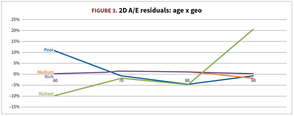
3. Identify pockets of good and poor model performance. Even if you can’t fix it, you can use this info in future UW decisions. I really like one- and two-dimensional views (e.g., age x pension amount) and performance across 50 or 100 largest plans—this is the precision level at which plans are actually quoted. (See Figure 3.)
What size of unexplained A/E residual is satisfactory at pricing segment level? How often will it occur in your future pricing universe? For example, 1-2% residual is probably OK. Ten to 20% in a popular segment likely indicates you have a model specification issue to explore.
Positive residuals mean that actual mortality data is higher than the model predicts (A>E). If the model is used for pricing this case, longevity pricing will be lower than if you had just followed the data, leading to a possible risk of not being competitive. Negative residuals mean A<E, predicted mortality being too high versus historical data, and a possible risk of price being too low.
4. Don’t forget about economic significance besides statistical significance. If model performance at very old or very young ages doesn’t matter to pension plans, feel free to sacrifice it to improve performance at ages that matter most for your pricing exercise. If calibrated to a sufficient amount of data, model fit for most popular plan types and richest pension amounts have the highest economic significance. In Figure 3, I would be mostly concerned about model fit for the richest cohort for ages 70 and 80. I would be less concerned about lower amounts, or more extreme ages.
If you make sure that the amount-weighted A/E = 100%, just in case your model missed some important predictors, the model will be correct in aggregate from the economic perspective.
5. Overfitting. Do you need all your variables? This is a very popular topic for those working with big data. Odds are all basic variables that you a priori expect to have an effect (age, gender, benefit amount) will not be eliminated through overfitting tests. With that said, Akaike information criterion (AIC) is a good test. Testing performance out of a sample is also good and there are a few flavors of how this can be done. Lastly, check that predictions are stable if you add one year of historical data. This will happen to you next year, after all, and you may want to avoid surprises.
Conclusion
As you can see, there is a lot of room for actuarial judgment, and we haven’t even scratched the surface on the application to UW of individual plans with more nuanced or missing data. For example, a case that recently has undergone a lump-sum election exercise will have some antiselection risk that should wear off over time. Or, what to do if some of the information fields are missing for a given plan?
I hope this was insightful and entertaining in a niche, actuarial kind of way. I also hope this inspires further learning, as it is impossible to cover everything in a short article. Even if you are a grand master of the latest predictive techniques and biggest data sets, never forget to apply common sense. Understand your data limitations, walk with GLM before you run with more complex models, learn to explain technical concepts in plain English, and strive for end-user satisfaction. (In case you are still wondering, this is a pretty tall order.) Good luck!
Lenny Shteyman, MAAA, FSA, CFA is an actuary at MetLife and can be reached at leonid.shteyman@metlife.com.